Colormaps for glaciology, packaged for Matplotlib.
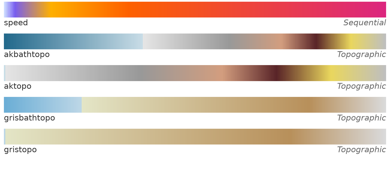
| Name | Type | Intended use |
|---|---|---|
speed |
Sequential | Ice surface speed |
akbathtopo |
Topographic | Bathymetry and surface elevation, Alaska |
aktopo |
Topographic | Surface elevation (land only), Alaska |
grisbathtopo |
Topographic | Bathymetry and surface elevation, Greenland |
gristopo |
Topographic | Surface elevation (land only), Greenland |
Contributions are welcome. Do you have a favorite colormap for ice thickness? Please let us know.
python -m pip install cmglaciologyFor the development version:
python -m pip install git+https://github.com/pism/cmglaciology.gitor, from a clone:
python -m pip install -e .import cmglaciology.cm as cmg
import matplotlib.pyplot as plt
import numpy as np
x = np.linspace(0, 1, 100)[np.newaxis, :]
plt.imshow(x, aspect='auto', cmap=cmg.speed)
plt.axis('off')
plt.show()For a reversed colormap, append _r to the colormap name:
plt.imshow(x, aspect='auto', cmap=cmg.speed_r)For a discretized colormap, use the
.resampled
method on any of the colormaps:
plt.imshow(x, aspect='auto', cmap=cmg.speed.resampled(25))Alternatively, the registered name string can be used. Names are prefixed
with cmg.:
import cmglaciology  # required in order to register the colormaps with Matplotlib
...
plt.imshow(x, aspect='auto', cmap='cmg.speed')
plt.imshow(x, aspect='auto', cmap='cmg.speed_r')
For an image of all the available colormaps:
from cmglaciology import show_cmaps

show_cmaps()
To also see how the colormaps look with a color vision deficiency, pass
cvd=True. This needs the
colorspacious package, which the
cvd extra installs:
python -m pip install "cmglaciology[cvd]"show_cmaps(cvd=True)simulate_cvd returns a single colormap as it is seen with a deficiency, to
use in a plot of your own:
from cmglaciology import simulate_cvd

plt.imshow(x, aspect='auto', cmap=simulate_cvd(cmg.speed, "deuteranomaly"))The colormaps were designed in QGIS against data values, so their color stops are not evenly spaced. The stops are (data value → position in the colormap is linear between the first and last value):
speed: 10, 30, 100, 250, 750 (m/yr)akbathtopo: -2000, 0, 1, 1250, 2000, 2500, 3000, 3500 (m)aktopo: 0, 1, 1250, 2000, 2500, 3000, 3500 (m)grisbathtopo: -500, 0, 1, 1500, 2000 (m)gristopo: 0, 1, 1500, 2000 (m)
To reproduce the QGIS rendering, use vmin/vmax equal to the first and last
stop. The topographic maps have a sharp break at sea level (0–1 m).
- Export the color ramp from QGIS (Layer Properties → Symbology → Save color
map to file) and put the file in
qgis/. - Run
python scripts/qgis2txt.pyto regenerate the 256-level RGB tables incmglaciology/cmaps/. - Add the name to one of the groups at the top of
cmglaciology/cm.py. - Run
python cm.pyfrom thecmglaciology/directory to refreshcolormaps.png,python scripts/show_cvd.pyto refreshcolormaps_cvd.png, andpytestto check everything.
Development happens on main; releases are cut from the release branch by
the ASFHyP3 actions workflows in
.github/workflows/, as in pism-terra:
- Every pull request to
mainadds an entry to CHANGELOG.md under a heading with the next version number, e.g.## [0.2.0](or carries thebumplesslabel if it changes nothing a user would notice). - To release, open a pull request from
maintoreleaseand give it one of the labelsmajor,minor,patchorbumpless. - Merging it tags the new version (
v0.2.0), which creates a GitHub release with the matching changelog section as its notes, bringsreleaseback intomain, and publishes the package to PyPI.
The version number of an installed package comes from the git tags, through
setuptools_scm.
The structure of this package — one text file of RGB values per colormap,
loaded and registered with Matplotlib on import, with reversed _r versions
and a show_cmaps() overview — is taken from
cmcrameri by Callum Rollo and
contributors, which packages Fabio Crameri's
Scientific colour maps.
cmglaciology/cm.py and the tests are adapted from cmcrameri's code, which is
distributed under the MIT License, Copyright (c) 2020 Callum Rollo. Many
thanks to Callum and the cmcrameri contributors for making this so easy to
reuse. Any errors in this adaptation are our own.
No colormap data from cmcrameri or the Scientific colour maps is included here. If you need perceptually uniform colormaps, use cmcrameri directly.
MIT, see LICENSE.txt.
The colormaps as they are seen with normal vision and with protanopia, deuteranopia and tritanopia, in which the red, green or blue cones do not work:
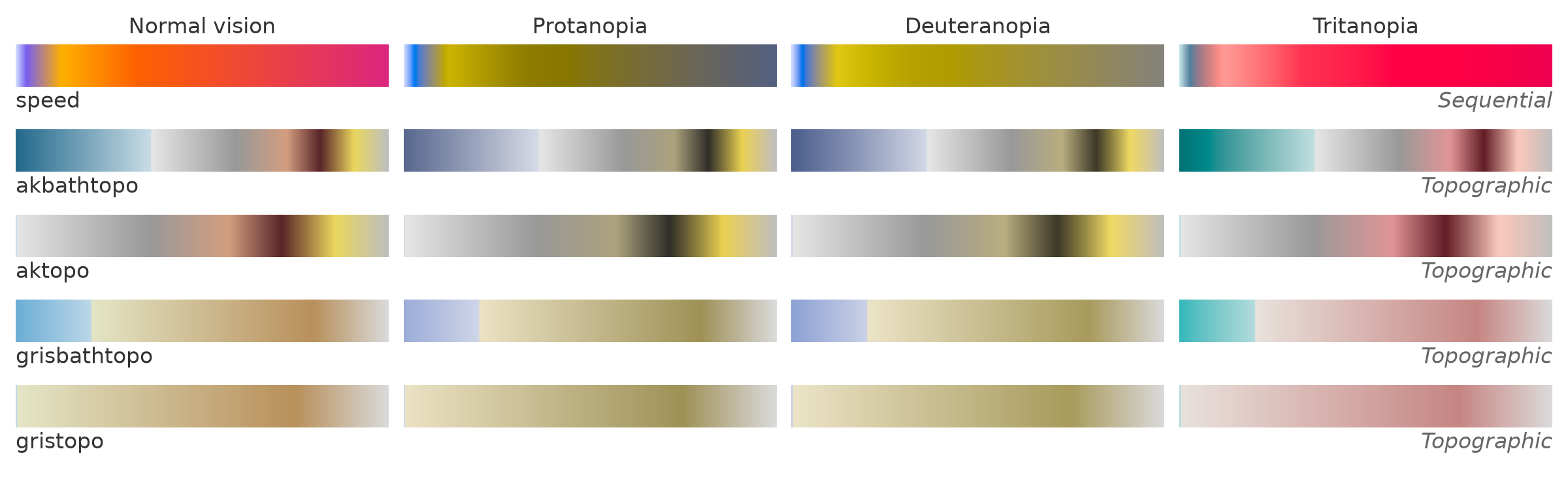
The figure is made with show_cmaps(cvd=True), by python scripts/show_cvd.py.
The simulation follows Machado et al. (2009), as implemented in
colorspacious. With protanopia and
deuteranopia, the orange-to-magenta upper part of speed turns into a single
olive ramp, so high speeds are harder to tell apart.
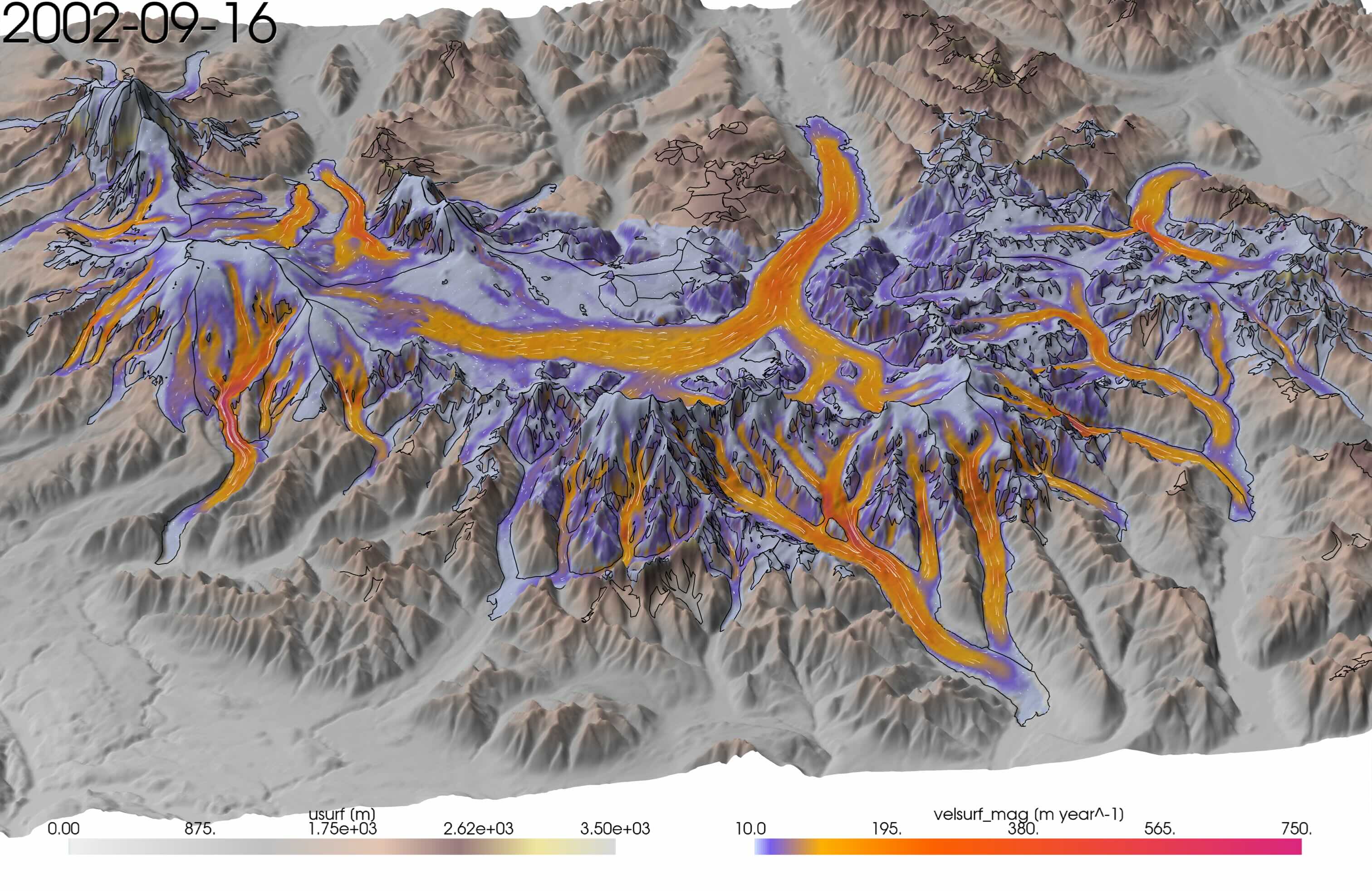
Example of Kennicott Glacier, Alaska, using aktopo and speed colormaps, rendered with pyvista: