Repository navigation
Data Sources and Math
- 🗄️ Data Source (data_source)
- 🎚️ On-Card Pickers (Points/Hour & Group By)
- 🧲 Raw Grouping (group_by: raw)
- 🔀 Value Transform
- 💶 Cost View (price_entity)
- ➖ Two-Entity Math (ref_entity)
- 📏 Range Band
- 〽️ Moving Averages
- 🕳️ Break on Gaps
- 📡 Attribute Data Source
- ☀️ Energy Dashboard Solar Forecast
- 🔌 External Statistics
🗄️ Data Source (data_source)
Home Assistant keeps two copies of most sensors: raw recorder history (every recorded sample) and long-term statistics (5-minute summaries). The data_source option chooses which one the card fetches — for the whole card or per entity:
type: custom:statistics-graph-chart-card
data_source: statistics      # card-wide preference
entities:
  - entity: sensor.power_meter
  - entity: sensor.grid_voltage
    data_source: history     # this entity keeps raw samples
An entity-level data_source overrides the card-level one; entities without their own setting follow the card. This is a YAML option — there is no editor control for it.
| Value | What you get | When to use it |
|---|---|---|
auto (default)
|
The card decides per entity and window — including the high-frequency detection below. | Almost always. Leave it alone unless a specific series needs forcing. |
statistics |
5-minute long-term statistics — roughly 50× less data for chatty sensors, so fetches are far cheaper and faster. Values track raw history closely but are not tick-identical, and averages are weighted by time (see below). | Power meters, CPU load, network counters — anything that updates every few seconds, especially over long windows. |
history |
Raw recorder history — every individual sample, exactly as recorded. | You need exact raw values or detail finer than 5 minutes. |
On raw history — cards of 24 hours or less, data_source: history, and date-picker day views — a bucket's avg, mean and median are computed over the readings recorded inside that bucket, each reading counting once. Home Assistant records a sensor only when its value changes, so a value held for 59 minutes and then changed once has no reading inside that hour's bucket: the hour shows the new reading only. Long-term statistics are summarised by Home Assistant with every value weighted by how long it was valid, so the same hour on a statistics-fed card — a window over 24 hours, a calendar grouping, data_source: statistics, or a sensor that fell back to statistics for a refresh — shows the time-weighted value, close to the held one. Sensors that report at a steady pace give the same number either way; sensors that change rarely can show a different average when a card crosses the 24-hour switch, and the legend's Avg follows the plotted buckets. This is the convention most history-based cards share. Set data_source: statistics on the card or entity if you want Home Assistant's time-weighted means on every window.
Raw history is requested over the WebSocket connection, the same way Home Assistant's own history cards fetch it; only a Home Assistant build too old to know that command falls back to the REST history API. (v4.03)
Under auto, the card watches what its history queries actually return. When one comes back flood-sized — a window of at least 6 hours whose response holds more than 5,000 rows and more than 200 rows per hour (thresholds v4.03) — the card marks that sensor as high-frequency, switches it to the statistics source on the spot, and remembers the decision in your browser for a week, so the expensive query only runs once. A one-time console note reports which sensor was switched.
A flagged sensor still falls back to raw history whenever you ask for finer detail than statistics can give — a window of 12 hours or less bucketed below the 5-minute statistics period. Each card decides for itself, so a close-up card keeps its full detail while day and week cards on the same sensor keep the cheap statistics path. (v4.03)
To keep raw samples for a sensor anyway, set data_source: history on that entity — explicit data_source settings always win over the detection.
When a series comes from long-term statistics and change_ignore_zero is on, the per-bucket change is recomputed from the statistics state column so that a counter's transient 0 readings are not re-counted as consumption. (v4.03) That recomputed value can never exceed Home Assistant's own change for the same row, so the card never reports consumption Home Assistant did not count. Periodic utility meters — helpers with a meter_period, or any sensor whose state column keeps dropping between rows — use Home Assistant's change directly, because their state is a per-period counter rather than a running total; cumulative counters keep the transient-zero protection.
🎚️ On-Card Pickers (Points/Hour & Group By)
Change the data resolution and the bucketing strategy directly on the card — no editor round-trip.
type: custom:statistics-graph-chart-card
show_pph_picker: true
show_group_by_picker: true
group_by_picker_position: right
entities:
- entity: sensor.power- Each dropdown starts on Auto (…), showing your configured value; picking anything else overrides it for this card only.
- Selections persist across reloads and take priority over Auto Scale while active.
- The Group By picker offers Interval, Hour, 2H / 3H / 4H / 6H / 12H, Date, Week, Month and Year.
Each picker has its own, fully independent sync group — same mechanism as date_picker_group:
# Controller card
show_pph_picker: true
pph_picker_group: page

# Receiver cards — no picker shown, still follow
pph_picker_group: page
pph_picker_group and group_by_picker_group don't interact: a card can follow one page-wide resolution group and a different bucketing group (or none).
General Settings → Overlay tab → Card Overlays → Points/Hour Picker and Group By Picker rows. The Group fields are always editable, even while the toggles are off.
🧲 Raw Grouping (group_by: raw)
group_by: raw turns bucketing off entirely: every recorded sample is drawn at its exact timestamp, with no averaging and no resampling — points_per_hour is ignored.
type: custom:statistics-graph-chart-card
group_by: raw
hours_to_show: 24
entities:
  - entity: binary_sensor.front_door
    name: Front Door
    graph_type: step
    state_map:
      - value: "off"
- value: "on"- Step charts of binary / state sensors — a door, pump, or heating-demand signal changes state at precise moments; bucketing smears those edges. Raw mode preserves every transition exactly where it happened.
- Sensors that record few, meaningful samples where a value interpolated into buckets would be misleading.
The Group By dropdown offers "Raw (no grouping)" whenever at least one entity uses graph_type: step — and always when the config already contains group_by: raw.
🔀 Value Transform
Apply a JavaScript expression to every data point before graphing. The transform has access to the current value and series-level statistics, making it possible to normalize, compare, and reshape data in ways that weren't possible before.
| Variable | Description |
|---|---|
x |
Current data point value |
first |
First value in the visible time window |
last |
Last value in the visible time window |
min |
Minimum value across the series |
max |
Maximum value across the series |
avg |
Average value across the series |
index |
Position of the current point (0, 1, 2…) |
All variables are computed after value_factor is applied, before the transform runs.
Display cumulative meter readings as relative consumption starting from zero:
entities:
  - entity: sensor.gas_meter
    value_transform: "return x - first;"
A gas meter reading 2200, 2210, 2225, 2240 becomes 0, 10, 25, 40.
A common use case: a single power sensor reports positive values for export and negative values for import. Use two entity entries with different transforms to separate them:
entities:
  - entity: sensor.grid_power
    name: "Grid Export"
    color: "#2ecc71"
    value_transform: "return x > 0 ? x : 0"

  - entity: sensor.grid_power
    name: "Grid Import"
    color: "#e74c3c"
value_transform: "return x < 0 ? -x : 0"| Expression | What it does |
|---|---|
return x - first |
Normalize to zero (cumulative → relative) |
return ((x - first) / first) * 100 |
Percentage change from start |
return (x - min) / (max - min) |
Min-max normalization (scale to 0–1) |
return x - avg |
Deviation from average |
return x > 0 ? x : 0 |
Keep only positive values (zero out negatives) |
return x < 0 ? -x : 0 |
Keep only negative values, flip to positive |
return Math.abs(x) |
Absolute value |
return x * 1.1 |
Add 10% markup |
return x - 273.15 |
Convert Kelvin to Celsius |
return (x * 9/5) + 32 |
Convert Celsius to Fahrenheit |
return Math.round(x / 100) * 100 |
Round to nearest hundred |
return x > 8 ? x : null |
Show the series only while it is above 8 |
return t <= now ? null : x |
Hide a forecast's past, keep only what is still ahead |
return t > now ? null : x |
The other half: actual data up to now, nothing after |
return (hour >= 17 && hour < 21) ? 8 : 12 |
A cap line that steps with the time of day |
return weekday <= 5 ? x : null |
Weekdays only |
Besides the value variables, the expression also receives four read-only time variables:
| Variable | Meaning |
|---|---|
t |
This point's timestamp, in milliseconds |
now |
The current time, in milliseconds |
hour |
Hour of this point as a decimal, 0–23.99 (so 17:30 is 17.5), in the card's display timezone |
weekday |
ISO weekday of this point: 1 = Monday … 7 = Sunday |
They make a per-entity time filter possible without a template entity — pair them with return … : null to draw a series only over the part of the X axis you want. An expression that uses now is re-evaluated about once a minute, so a t <= now cut-off keeps up with the clock on its own.
If your expression declares its own
t,now,hourorweekday— withvar,let,const, or as a function parameter — the card compiles it without the time variables so your own names keep working exactly as before.
Entity → Advanced tab → Advanced Calculations → Value Transform — a monospace text input field. Enter the expression directly (e.g., return x - first).
- The expression must be valid JavaScript and include a
returnstatement - Returning
nullleaves a visible gap at that point: the line breaks there rather than joining across the hole, and the tooltip, moving averages and range band all respect it. An expression that throws or returns a non-number does the same — it is never silently replaced by the original value (changed in v4.04 — these points used to be removed, which let the line connect straight over them) - Applied to every data point individually — both historical and live values
- Works with all chart modes, aggregation functions, and other entity options
- Context variables (
first,min, etc.) are only available when processing a full data series — in the state row live value display, all context variables equalx
💶 Cost View (price_entity)
Multiply a series by the value of another entity over time — turn a kWh consumption chart into a money chart using a dynamic price sensor (Nordpool, EPEX, Tibber, a utility tariff helper). Per-entity price_entity needs no template sensor and no duplicate entity: the card bills the consumption itself.
type: custom:statistics-graph-chart-card
card_header: Energy Cost
hours_to_show: 168
group_by: date
entities:
  - entity: sensor.energy_meter
    name: Cost
    graph_type: bar
    aggregate_func: change
    price_entity: sensor.electricity_price
    unit: "€"
decimals: 2- The price is read as a step function from the price entity's own history — each price is valid from the moment it was recorded until the next change. Long windows automatically use long-term statistics (hourly mean) for the price series.
- The multiplication happens per consumption slice, before bucketing — every slice of consumption is billed at the price that was active at that moment, so each bucket is the exact sum Σ(valueᵢ × priceᵢ).
- Designed for
aggregate_func: changeon cumulative energy counters — setunitto your currency so the state row, tooltip, and axis all read as money. -
price_attributereads an attribute of the price entity instead of its state — dot notation is supported for nested paths (e.g.raw_today.0.value). - A state change of the tariff entity auto-refreshes the card, so a price update redraws the cost immediately.
- Period Comparison ghosts are billed at their own period's prices — last week's ghost uses last week's tariffs, keeping the comparison honest.
- Not applied to
fixed_valueordata_attributeentities.
Multiplying the period's total consumption by the average price is only correct when consumption is flat. With time-of-use tariffs the expensive hours tend to be exactly the high-consumption hours, so average × total systematically misstates the bill. Billing every slice at its own momentary price reproduces what the utility actually charges.
Entity → Advanced tab → Advanced Calculations → Price Entity and Price Attribute inputs.
➖ Two-Entity Math (ref_entity)
Plot the combination of two entities — most often their difference — without creating a template sensor. ref_entity names the second entity and ref_op says how to combine them:
type: custom:statistics-graph-chart-card
hours_to_show: 24
entities:
  # indoor − outdoor, the classic delta. ref_op defaults to subtract,
  # and with no name: the series is labelled "Indoor − Outdoor" automatically.
  - entity: sensor.indoor_temperature
    ref_entity: sensor.outdoor_temperature

  - entity: sensor.solar_production
    name: Net export
    ref_entity: sensor.house_consumption
    ref_op: subtract

  # the reference can come from an attribute (e.g. a weather entity)
  - entity: sensor.pool_temperature
    ref_entity: weather.home
    ref_attribute: temperature
ref_op: divideThe reference entity's own history is fetched alongside your data and read as a step function: every sample of the main entity is combined with the reference value that was valid at that moment. The math runs before bucketing, so avg over a bucket is the average of the difference, and min/max are the smallest/largest instantaneous gap — not min(A) − min(B). With a delta aggregation (change, diff, sum, delta), subtract / add / reverse_subtract (v4.03) and divide / reverse_divide by a meter (v4.07) combine the two entities per bucket instead — see the next section.
-
Reversed operators.
reverse_subtractgivesB − Aandreverse_dividegivesB ÷ A. This is not the same as swapping the two entity ids: the main entity supplies the timeline the reference is sampled onto, plus the unit, aggregation, data source, colour and offset. Keep the better-sampled sensor asentity:and flip the arithmetic instead (e.g.COP = heat ÷ powerwhilepowerstays the main series). -
subtract/add/reverse_subtractcombine levels — or, with a delta aggregation, whole buckets. Withavg,min,max,last,firstormedianthe reference is sampled at each of the main entity's readings. Withchange,diff,sumordelta(v4.03) the two entities are first aggregated the same way (for statistics-fed series that is Home Assistant's own per-periodchange), then combined per bucket — the way to add two daily-production meters into one monthly total:entities: - entity: sensor.goodwe_today_s_pv_generation name: Total production ref_entity: sensor.solaredge_production_today ref_op: add aggregate_func: sum graph_type: bar group_by: month
A bucket in which one side has no data counts that side as 0, so a month with only one inverter reporting still shows the other's production;
price_entityis applied to both sides. The bucket-wise path needs anentity:series in a bucketed chart — astatistic_id-only or attribute series still renders empty with a console warning.multiply, anddivideby a level (a constant, aninput_number, a price, ameasurementsensor), are allowed with every aggregation — that is exactly whatprice_entitydoes. -
divide/reverse_divideby a meter — total ÷ total per bucket. (v4.07) When the reference is a meter — itsstate_classistotalortotal_increasing(energy, gas, water) — and the aggregation ischange,diff,sumordelta, both entities are first aggregated the same way and then divided per bucket. A heat pump's daily COP is the day's heat output ÷ the day's electricity:entities: - entity: sensor.heat_pump_energy_output_heating name: COP ref_entity: sensor.heat_pump_electricity_used_heating ref_op: divide aggregate_func: change group_by: date unit: COP
A bucket where the divisor is 0 or has no data stays empty instead of showing an infinite ratio, a bucket where only the divisor has data shows 0, and a reference with no data at all leaves the series empty. By default the state row shows the newest bucket, so with
group_by: dateit reads today's ratio so far. Pie, radial bar, polar area, radar, ranking and waterfall charts, the heatmap and calendar cells and the state row'spctshare divide the totals of the whole window or cell the same way, so a week of daily COPs reads the week's COP instead of the sum of seven ratios; a bucket that stays empty because its divisor is 0 counts on neither side.price_entitymultiplies the main entity only (pricing both sides would cancel it out) — put the priced meter asentity:and usedivide: electricity with a tariff ÷ heat is the cost of one kWh of heat. The bucket-wise limits above apply here too. A reference that is a level — a constant, aninput_number, ameasurementsensor or anyref_attribute— keeps the sample-by-sample rule (energy ÷ floor area), andmultiplyalways combines sample by sample. -
Carry-forward, but nothing invented. The reference is held until it next changes — the same rule Home Assistant itself uses for a state, and the same one
price_entityfollows. That is what makes a step-shaped reference (a setpoint, aninput_number, a mode) work. What the card will not do is invent a value before the reference's first sample: that stretch is a gap. Since the card carries values across gaps by default, a reference that dies mid-window shows as a flat line — addbreak_on_null: trueif you would rather the line break there. -
Both operands should share a unit for
subtract/add; the result keeps the main entity's unit. Formultiply/dividesetunityourself. -
value_factorandinvertapply to the main entity only, before the combination. -
The state row and the trend arrow follow the combined series, not the bare main entity.
-
Not available on
data_attribute(forecast-array) orfixed_valuerows. -
Only one reference and one operator per entity. For multi-operand formulas (
A − B − C) you still need a template sensor — a general cross-entity expression is planned for a later release.
Note:
data_value_expression+data_varsdo not do this. They only apply to an attribute-array data source, anddata_varsresolves each name to the referenced entity's current state — a constant, not a series. Useref_entityfor math against another entity over time.
Editor: Entity → Advanced → Reference Entity, Operation, Reference Attribute.
📏 Range Band
The Range Band feature draws a shaded min/max area behind each line entity, showing how much the value fluctuated within each aggregation bucket.
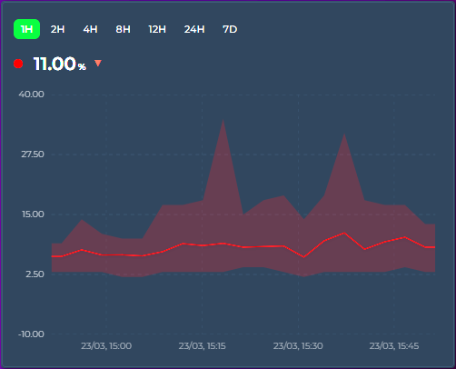
When points_per_hour aggregates multiple raw data points into a single graph point, the displayed value is typically the average (or whichever aggregate_func you've chosen). The range band shows the full min → max spread of raw values that were combined — so you can see both the trend and the volatility.
entities:
  - entity: sensor.outdoor_temperature
    show_range_band: true
    color: "#ff4757"
  - entity: sensor.indoor_temperature
    show_range_band: false
color: "#378ADD"- Temperature: narrow band = stable climate, wide band = fluctuating (e.g. HVAC cycling)
- Energy: see consumption spikes vs steady draw within each time bucket
- Sensor noise: distinguish real signal changes from noisy sensor readings
Entity → Graph tab → Line section → Range Band toggle (next to Data Points). Timeline mode only.
When hovering, an additional row shows the range: Range: 21.2 → 22.8 °C.
〽️ Moving Averages
Overlay one or more simple moving-average (SMA) lines on top of any entity — a smoothed trend line that averages the last N buckets. Add as many as you like, each with its own period, color, and width. Perfect for separating signal from noise on busy sensors (CPU load, power, prices) or for classic short/long crossover views (e.g. MA7 vs MA26).
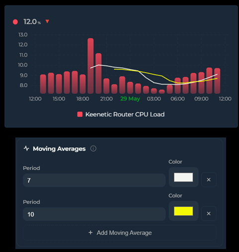
entities:
  - entity: sensor.keenetic_router_cpu_load
    graph_type: bar
    moving_averages:
      - period: 7          # short MA — averages the last 7 buckets
        color: "#ffffff"
        show_label: true   # draw a small "MA7" tag on the line
      - period: 26         # long MA — averages the last 26 buckets
        color: "#f1c40f"
        width: 2           # optional line thickness (px)
show_label: true # draw "MA26"Each line's period is a number of buckets, and the bucket size comes from the chart's timeframe — points_per_hour in interval mode, or group_by (hour / date / week / month / year). So with group_by: hour, period: 26 averages the last 26 hourly buckets (MA26). With points_per_hour: 12 (one bucket every 5 minutes), period: 26 covers the last ~130 minutes.
A 26-bucket average normally needs 26 buckets of history before it can produce its first value. If your visible window only holds a handful of buckets (e.g. hours_to_show: 24 with group_by: hour → 24 buckets), a plain MA26 would never have enough data to draw.
This card solves that by extending the history fetch backward automatically by the amount the longest moving average needs — independent of the visible window. The MA is computed over that extended range and then trimmed to the window, so MA26 draws fully across a 24-hour view without you having to widen hours_to_show or scroll. The visible chart, axis, statistics, and extrema are unchanged — only the moving-average lines use the extra look-back.
The look-back applies to entities whose data comes from History or long-term statistics. Synthetic sources (
fixed_value,data_attribute) average only what's in the window.
When the entity is drawn as candlesticks, each moving average uses the close of every candle (otherwise it averages the bucket value), so an MA over candles behaves like the moving averages on a trading chart.
Turn on show_label for any line to draw a small MA7, MA26 … tag right at the end of that line, so you can tell several averages apart at a glance:
    moving_averages:
      - period: 7
        color: "#ffffff"
        show_label: true
By default the label text is the period prefixed with MA (MA7, MA26, …). (v4.07) Give the item a name to print your own text instead — so a weekly average on hourly buckets reads Weekly trend rather than MA168:
    moving_averages:
      - period: 168
        show_label: true
        name: "Weekly trend"
name only changes the wording: show_label still decides whether a label is drawn, so a name without show_label: true draws nothing, a blank name falls back to MA<period>, and a short name reads best. Whatever the text, the label is drawn at the end of the line and clamped inside the chart, so it never spills outside the plot, with a subtle background halo so it stays readable over the line and the data. It's off by default — flip the Label switch next to the color picker, or set show_label: true in YAML.
- Each moving average is plotted against the entity's own Y axis, so it lines up with the bars / line / candles it summarizes.
- Lines render in their configured
color; leavecolorempty to fall back to a default.widthdefaults to a thin line. - Timeline mode only.
Per-entity → Graph tab → Moving Averages (just below the Graph card). Click Add Moving Average to add a line, set its Period and Color, flip Label to print an MA7-style tag on the line, type a Name (v4.07) to replace that tag with your own text (the field's placeholder shows the automatic MA<period> text; leave it empty to keep it), and use the ✕ button to remove one.
🕳️ Break on Gaps
When a sensor goes unavailable or unknown, the card normally keeps the line continuous by carrying the last known value forward across the gap. That's great for short blips (brief WiFi drops, bucket-level reporting irregularity) but can hide genuine multi-hour outages behind a flat line. The per-entity break_on_null option lets you opt in to a visible break instead.
entities:
  - entity: sensor.steady_sensor
    # default — continuous line, last known value carried across any gap

  - entity: sensor.flakey_sensor
    break_on_null: true
    # short blips still connect, but longer outages appear as gaps

  - entity: sensor.very_specific
    break_on_null: true
carry_forward_ms: 900000 # advanced — 15 min threshold| Setting | Effect |
|---|---|
break_on_null: false (default)
|
Carry-forward runs indefinitely within the visible window. No null-induced gaps, ever. The long-standing default behavior. |
break_on_null: true |
Short sample gaps (bucket-level blips, irregular reporting, brief drops) stay connected. Longer outages — default threshold min(3 × bucket width, 30 minutes) — appear as visible breaks in the line. |
carry_forward_ms: N (YAML, advanced)
|
Override the threshold with an explicit value in milliseconds. Applies regardless of the break_on_null setting. |
A pure "zero carry-forward" mode turns out to be too aggressive on real-world sensors. When bucket width is finer than the sensor's natural sample interval (a common setup at high points_per_hour), dozens of buckets between two real samples end up empty even though the sensor is perfectly healthy. The time-based threshold distinguishes "I'm waiting for the next sample" from "the device has been gone for a while" — which is the distinction users actually want to see.
Entity → Graph tab → Graph section → Break on Gaps toggle (next to Show Average and Data Labels). Shown in every chart mode — carry-forward affects the bucketed data, so it matters wherever those buckets are drawn.
Since v3.32 the editor hides options that do nothing for the selected chart mode, down to the individual field — a section disappears once everything inside it is hidden, a tab once all its sections are, and you are moved to the first surviving tab. Break on Gaps survives that pass in all fourteen modes, while a Timeline-only neighbour like Range Band does not. Nothing is lost either way: a hidden option keeps its YAML value and comes back when you switch modes again.
-
Changed in v3.25 — an empty bucket now carries the previous bucket's last recorded sample (its exit state) forward, not the previous bucket's aggregated value. With
aggregate_func: firstormax, a momentary spike no longer smears across the quiet buckets that follow it; withavg, the carried value is the last actual reading instead of the previous bucket's average. - Does not affect
value_transformscripts that returnnull— those buckets are already null before carry-forward logic runs, so they stay a visible gap either way. - Works independently per entity, so you can mix well-behaved sensors (continuous line) with flakey ones (visible gaps) on the same card.
📡 Attribute Data Source
Read chart data directly from an entity attribute instead of history. The attribute must contain an array of objects with time and value fields. The X-axis automatically extends into the future when data contains future timestamps.
Ideal for energy spot prices, weather forecasts, and solar production predictions. No history or statistics API calls are made for these entities.
entities:
  - entity: sensor.epex_spot_price
    data_attribute: data
    data_time_field: start_time
    data_value_field: price_per_kwh
    value_factor: 2
    graph_type: step
    name: "Electricity Price"
Common configurations:
| Integration | data_attribute |
data_time_field |
data_value_field |
|---|---|---|---|
| EPEX Spot | data |
start_time |
price_per_kwh |
| Nordpool | raw_today |
start |
value |
| Tibber | price_info |
startsAt |
total |
| Solcast PV Solar (HACS) |
detailedForecast (on the per-day forecast_today / forecast_tomorrow … sensors) |
period_start |
pv_estimate |
Not every forecast integration exposes an array. Core Forecast.Solar has no attributes at all — its forecast reaches only the Energy dashboard (
energy/solar_forecast). Open-Meteo Solar Forecast (HACS) exposes per-daywh_perioddictionaries (energy_production_today,_tomorrow,_d2…_d7), which are not arrays; merge them into one list with a template sensor ([{ start, wh }, …]) and pointdata_attributeat that. Or skip all of that:solar_forecast: trueon a row draws the Energy dashboard's solar forecast directly — see Energy Dashboard Solar Forecast below.
Compatible with existing value_factor, value_transform, aggregate_func, and group_by. The calendar group_by modes (hour, date, week, month, year) regroup the array when the requested cell is coarser than its native spacing — 96 quarter-hourly prices under group_by: hour become 24 hourly values combined with aggregate_func — and pass it through untouched otherwise, so an already-hourly array stays as published. interval (the default) and raw never regroup; the fixed 2h–12h modes are not supported for attribute arrays. points_per_hour does not apply — it controls fetching, and an attribute source fetches nothing. The time and value field names support nested paths via dot notation (e.g. forecast.0.temperature or integrated.0.value).
Sometimes the value you want isn't a single field — you need to combine several fields from each element, fold in other entities (fees, tax rates, tariffs), and apply a formula. Set data_value_expression instead of data_value_field: a small arithmetic expression evaluated for every array element, with the element's own fields in scope plus any names you map in data_vars.
entities:
  - entity: sensor.tibber_hourly_cost
    name: Electricity
    graph_type: bar
    data_attribute: nodes
    data_time_field: from
    data_time_unit: iso
    data_value_expression: "(unitPrice - unitPriceVAT) * 100 * consumption * (1 + mwst)"
    data_vars:
      mwst: input_number.vat_rate
data_vars maps a name to an entity ID; each resolves to that entity's numeric state and is re-evaluated live when it changes. Inside the expression you can use:
| In scope | Examples |
|---|---|
| Element fields |
unitPrice, consumption, … (any field of the array item) |
data_vars names |
mwst, base, … |
| Operators |
+ - * / % and parentheses ( )
|
| Functions |
min, max, abs, round, floor, ceil, sqrt, pow, coalesce (v4.08)
|
This is not JavaScript — there are no other variables, no property access, and no calls beyond those functions, so it can't run arbitrary code. If the expression is empty or fails to parse, the entity falls back to data_value_field.
Elements without a value (v4.08) — an array element that lacks the value field (or holds text that isn't a number) has no reading, so it draws no point: a bar is simply missing, and a line, area or step joins its neighbours — with line_shape: hv the last value is held until the next element. When a missing field means zero — a solar or charging plan that only lists the quarters with energy, for example — wrap the field in coalesce, which returns its first argument that is a number:
    data_attribute: plan
    data_time_field: tijd
    data_value_expression: "coalesce(zon_laden_kwh, 0)"
coalesce takes any number of arguments, so coalesce(override, price, 0) falls through a chain of fields, and it treats a division by zero or a data_vars entity that is unavailable as empty too. When every argument is empty the element is skipped, as before.
Because each element is evaluated independently, two entities reading the same array with different expressions stack cleanly — e.g. splitting an hourly energy cost into a consumption layer and a fixed-fee layer:
type: custom:statistics-graph-chart-card
stacked: true
group_by: hour
entities:
  - entity: sensor.tibber_hourly_cost
    name: Energy
    graph_type: bar
    data_attribute: nodes
    data_time_field: from
    data_time_unit: iso
    data_value_expression: "(unitPrice - unitPriceVAT) * 100 * consumption * (1 + mwst)"
    data_vars: { mwst: input_number.vat_rate }
  - entity: sensor.tibber_hourly_cost
    name: Fees
    graph_type: bar
    data_attribute: nodes
    data_time_field: from
    data_time_unit: iso
    data_value_expression: "(base/30/24 + grid/24 + meter/24) * (1 + mwst) * 100"
    data_vars:
      base: input_number.base_price_month
      grid: input_number.grid_fee_day
      meter: input_number.meter_fee_day
      mwst: input_number.vat_rate
Editor: Per-entity → Advanced tab → Attribute Data Source → Value Expression field, and Data Vars (one
name: entity_idper line).
By default, the time field is parsed as an ISO date string. Set data_time_unit to interpret it differently — perfect for sensors that expose monthly summaries, hourly profiles, day-of-year datasets, or Unix timestamps without generating artificial timestamps.
| Unit | Range | Behavior |
|---|---|---|
iso (default) |
string / epoch ms |
new Date(t) — existing behavior |
epoch_seconds |
number | Unix timestamp in seconds |
epoch_ms |
number | Unix timestamp in milliseconds |
month_of_year |
1..12 | First day of that month in data_time_year (default: current year) |
day_of_month |
1..31 | That day of the visible window's month, in data_time_year (default: the window's year). A value past the month's end is clamped to its last day |
day_of_year |
1..366 | That day in data_time_year
|
week_of_year |
1..53 | Monday of that ISO week in data_time_year
|
hour_of_day |
0..23 | That hour of today |
Example — a sensor exposing monthly yield expectations as [{Month: 1, Expectation: 320}, {Month: 2, Expectation: 489}, ...]:
type: custom:statistics-graph-chart-card
group_by: month
graph_start: year
hours_to_show: 8760
entities:
  - entity: sensor.sma_month_yield_expectation
    data_attribute: Expectation
    data_time_field: Month            # 1..12
    data_value_field: Expectation
    data_time_unit: month_of_year     # interpret as Jan..Dec
    graph_type: bar
    aggregate_func: max
Renders 12 bars labelled Jan–Dec on the X-axis. Tooltip shows the actual month + value. All other features (date picker, group_by, fill, theming) work normally because the parser converts the numeric category into a real Date internally.
Editor: Per-entity → Advanced tab → Attribute Data Source → Time Unit dropdown and Reference Year input
☀️ Energy Dashboard Solar Forecast
Draw the solar forecast your Energy dashboard already shows — Forecast.Solar, Solcast, Open-Meteo Solar Forecast or any other integration that feeds the dashboard — as a row of this card. No entity, template sensor or attribute array is needed: the card reads the same forecast the Energy dashboard reads (energy/solar_forecast).
entities:
  - solar_forecast: true          # no entity / statistic_id needed
    name: "PV forecast"
    graph_type: line
line_style: dashed-
What you get: hourly points in kWh (the forecast is energy per hour), as far back as the integration returns them (Open-Meteo keeps about three months of past hours, Forecast.Solar starts today) and as far ahead as it forecasts.
aggregate_funcdefaults tosumandunittokWh; override either like on any row (unit: W+value_factor: 3plots the hourly mean power — an hourly Wh value is numerically the mean W of that hour). -
Sources: by default every solar source of the Energy dashboard that has a forecast configured is summed per hour, the way the dashboard draws it.
solar_forecast_source: sensor.pv_a_energy(the source's energy-production statistic) draws one source only. The row is named after the source (Energy dashboard name or friendly name + " forecast"), or Solar forecast;name:overrides as usual. -
Daily totals:
group_by: date(orweek/month) sums the hours into calendar cells — the right view for a week or month card. -
Window: the row follows the card window like an attribute source. A rolling window (
hours_to_show) is stretched to the last forecast hour — about 16 days ahead with Open-Meteo.graph_start: day|week|monthends at now unless you addshow_full_period: true, which shows the whole period including the hours ahead. Withenergy_date_syncor the built-in date picker the current period also ends at now and is then stretched to the last forecast hour; addshow_full_period: trueto stay on the selected period (today, this week, this month) with the forecast clipped to it. Past periods show the past hours the integration returns.auto_scale_pointssteps aside for a solar forecast row, exactly as it does fordata_attribute. -
State row: shows the forecast of the current hour (today's total under
group_by: date);primary_state_as: sumshows the total of the window,lastthe last forecast hour. -
Nothing to draw? If the Energy dashboard is not configured, no solar source has a forecast, or the forecast integration is not loaded, the row stays empty, one warning is written to the browser console and the detail legend notes it. The forecast refreshes with the card's periodic poll (every 5 minutes, 15 with a calendar
group_by) or withupdate_interval.
Day view — hourly forecast next to the real production:
type: custom:statistics-graph-chart-card
graph_start: day
show_full_period: true
show_legend: true
entities:
  - entity: sensor.pv_energy_today
    aggregate_func: change
    graph_type: bar
    unit: kWh
  - solar_forecast: true
    name: Forecast
    graph_type: line
    line_style: dashed
Week view — one bar per day, one source only:
type: custom:statistics-graph-chart-card
graph_start: week
show_full_period: true
group_by: date
entities:
  - solar_forecast: true
    solar_forecast_source: sensor.pv_a_energy
    graph_type: bar
Following the Energy dashboard's own date picker:
type: custom:statistics-graph-chart-card
energy_date_sync: true
show_full_period: true     # stay on the selected period; without it the window ends at now and is stretched to the last forecast hour
group_by: date
entities:
  - solar_forecast: true
Past days: the hours before now are whatever the forecast integration returns today for those hours — not a copy of the forecast that was shown on that day. Use them for context, not for accuracy tracking.
Editor: Per-entity → Advanced tab → Solar Forecast (Energy Dashboard) → Solar Forecast toggle and the Forecast Source dropdown (the dashboard's solar sources that have a forecast, by name; All solar sources is the default). The Entity picker on the General tab is marked optional while the toggle is on; Aggregation shows Sum and the Unit field hints kWh.
🔌 External Statistics
Display data from imported statistics that don't have a regular entity in Home Assistant. This covers energy data from integrations like Gazpar, Linky, Tibber, and others that import directly into HA's statistics database.
Some HA integrations don't create sensor.* entities. Instead, they write data directly into the statistics and statistics_meta database tables using HA's async_import_statistics() API. These statistics have IDs with a colon separator (e.g. gazpar:gazpar_consumption) and are visible on the Energy dashboard and the built-in Statistics Graph card, but not in the entity registry.
Use statistic_id instead of (or alongside) entity:
entities:
  - entity: ""
    statistic_id: "gazpar:gazpar_consumption"
    name: "Gas Consumption"
    color: "#f39c12"
    aggregate_func: sum
  - entity: ""
    statistic_id: "linky:linky_consumption"
    name: "Electricity"
    color: "#378ADD"
    aggregate_func: sum
  - entity: sensor.indoor_temperature
    name: "Temperature"
    color: "#ff4757"
You can mix external statistics with regular entities on the same card.
- The card detects external statistics by checking for a
:in thestatistic_id - Data is fetched via HA's
recorder/statistics_during_periodWebSocket API — the same API the Energy dashboard uses - Since there is no live state, the state row displays the last known value from the statistics data
- All card features work: tooltip, legend, axes, stacking, offset, zoom, color thresholds, etc.
Entity → General → Statistic ID input field (monospace, below the entity picker). Set the entity picker to empty and fill in the statistic ID.
- Go to Developer Tools → Statistics in HA
- Search for the integration name (e.g. "gazpar")
- The statistic ID is shown in the list (e.g.
gazpar:gazpar_consumption)